The basics of the amplification curve
All posts · · J.M. Ruijter & Maurice van den Hoff
This is the first blog in a series discussing different aspects of PCR analysis. To start at the very basics, PCR, short for polymerase chain reaction, is a molecular process in which a DNA target is exponentially amplified. PCR can be described mathematically by the equation . Or in words: the number of target copies after cycles () is the number of copies at the start () of the reaction times the efficiency of the PCR () to the power of the number of cycles (). An efficiency of corresponds to 100% efficiency, a perfect doubling of the target every cycle. A graph of the amplification data should therefore show an exponential increase.
Why the logarithmic Y-axis matters
The progress of the PCR is monitored with fluorescent dyes or probes. Before the cycling starts, the reaction components already fluoresce, which is referred to as baseline fluorescence (), and as a consequence the observed fluorescence at cycle () is described with the equation . is thus the sum of the amplification-independent baseline fluorescence () and the amplification-dependent fluorescence (). Although the fluorescence value should increase close to twofold in each cycle, the observed fluorescence, plotted on a linear Y-axis versus the cycles on the X-axis, displays a sigmoidal curve. A typical amplification curve starts close to zero and stays there for about halfway the PCR, then shows a sharp sudden increase and subsequently reaches a constant plateau, at which it stays till the last cycle (Fig. 1).
On a logarithmic Y-axis, the raw fluorescence data also show such an S-shaped amplification curve. This S-shaped curve is because the fluorescence due to the amplified product is too low to be visible above the baseline fluorescence. Although this phase is often referred to as the ground phase, its last cycles may already contain amplification-dependent fluorescence.

Baseline correction is where analysis starts
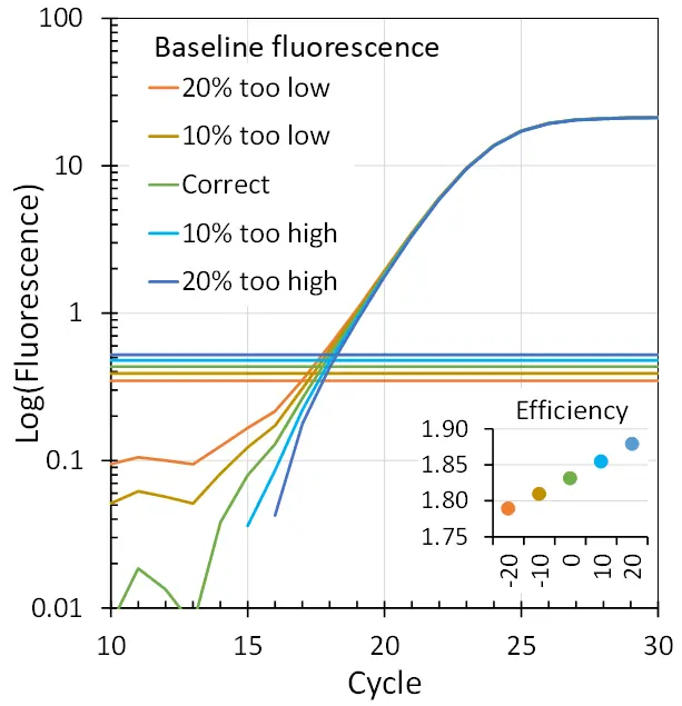
The analysis of qPCR data, therefore, has to start with the removal of the contribution of the baseline fluorescence from the observed data. Conversion of the kinetic equation of PCR to its logarithmic form gives , which is in fact the equation of a straight line. On a logarithmic Y-axis, the baseline-corrected fluorescence values will thus show as a graph in which the exponential phase of the reaction is a straight line. Or, the other way around: when the baseline fluorescence is correctly estimated and subtracted from the observed data, the graph of the corrected fluorescence data will show as a straight line, which is the exponential phase. Seeing this straight phase can thus be used as a visual criterion for the accuracy of the baseline subtraction (Fig. 2).
When the data points of the log-linear phase are not on a straight line, the estimated baseline value was too high or too low. Moreover, the amplification curves of all reactions amplifying the same target should, in principle, be parallel. Amplification curves with a deviating slope indicate the presence of inhibitors or stimulators in the biological sample, or a sample with sequence mismatches due to SNPs in the primer binding sites, or errors in the composition of the reaction mixture. As described below, each of these variables will affect the amplification efficiency, as determined from the slope of the exponential phase.
How instrument software gets the baseline wrong
The baseline fluorescence that is determined and subtracted by the software of the qPCR instrument uses an algorithm that fits a trendline through the observed fluorescence values from a user-defined number of early ground phase cycles. This results in a cycle-dependent baseline fluorescence. These early fluorescence values are the lowest observed in the entire PCR run and are prone to random noise. Consequently, these trendlines may have random directions that are extrapolated to all cycles till the end of the PCR, often resulting in increasing or decreasing plateau levels.
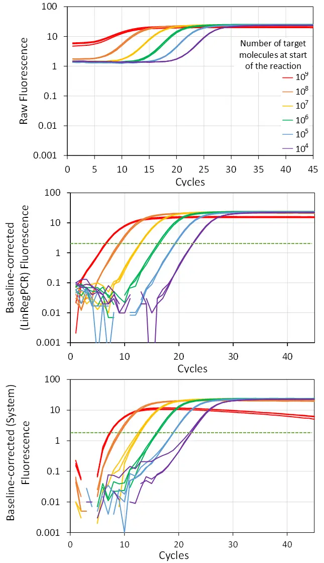
Another caveat in using the early cycles of the reaction to estimate the baseline fluorescence arises when the target is present in very high numbers at the start of the reaction. In such a case, the observed fluorescence in the first cycles, due to the high number of targets in the reaction, will be in the exponential phase and sometimes already close to the plateau fluorescence. Because the algorithm considers this early fluorescence to be baseline fluorescence, its value is subtracted from all following cycles, with often disastrous results: in the worst scenario, a very positive sample is interpreted as a negative one (Fig. 3).
The LinRegPCR approach: fit from the plateau down
To eliminate the effect of erroneous baseline correction based on too early cycles, the baseline estimation algorithm implemented in our LinRegPCR program uses an iterative approach to find, for each reaction individually, the fluorescence baseline value that yields the longest continuous range of data points in the exponential phase of the amplification curve. In this implementation, the early cycles do not play a role because the iterations start from the end of the exponential phase and progress downward. However, for this algorithm to work, the reaction has to reach the plateau phase. When this is not the case, the user should repeat the PCR run with more cycles.
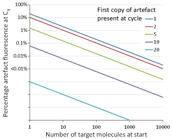
It is often argued that too many PCR cycles will increase the amplification of artefacts. However, it can be easily shown that for an artefact to make a substantial contribution to the observed fluorescence, it should occur in, or even before, the first cycles of the run. Artefacts that only occur in the last PCR cycles are very low in concentration compared to the amplicons already present in those cycles and as such have a minute effect on the outcome of qPCR analysis (Fig. 4).
Why assay optimisation is a trade-off
A high baseline fluorescence value will substantially decrease the number of data points that will be available between baseline and plateau. To reliably analyse the amplification curve, there should preferably be at least four data points in its exponential phase. The optimisation of the assay should, therefore, aim for a low baseline fluorescence. However, when the primer concentration is lowered to reduce the baseline fluorescence, the amplification efficiency as well as the plateau level will also be reduced. Assay optimisation therefore is a trade-off between baseline value, plateau level, and amplification efficiency.
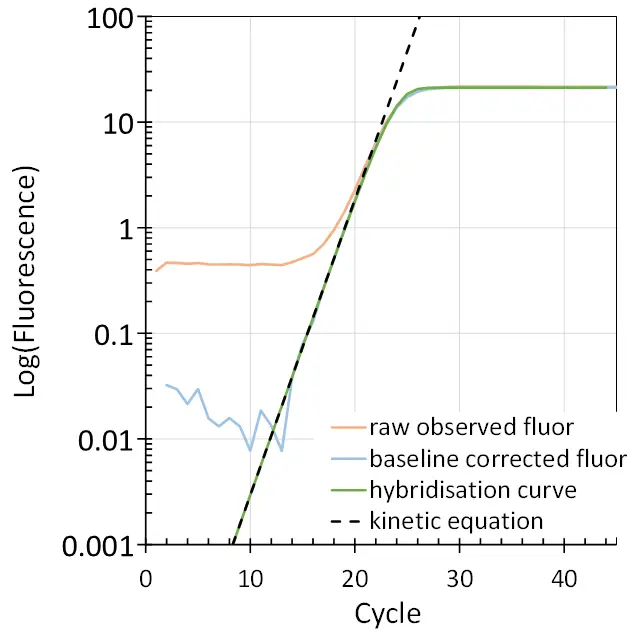
Although the amplification curve is expected to be a straight line when plotted on a logarithmic Y-axis, in practice one sees a bending down towards the plateau phase in the late cycles. In this transition phase, the cycle-to-cycle increase of the amplicons starts to decrease until the reaction reaches a constant plateau level. This decrease in efficiency is determined by the hybridisation kinetics, which are governed by the decreasing concentration of primers and increasing concentration of amplicons. When the reaction reaches this cycle number, the increasing number of amplicon-amplicon hybrids starts to hamper the number of primer-amplicon hybrids formed during the annealing phase of the PCR. The decrease in primer-amplicon hybrids then results in a less pronounced increase of amplicon number per cycle and thus in a decrease in the observed amplification efficiency.
This decrease in efficiency occurs when the amplicon number reaches 1% of the initial primer concentration. Because of the enormous excess of primers at the start of the PCR, the efficiency can be considered constant till that cycle. Fitting of the hybridisation equation to the observed fluorescence data indeed shows that until that cycle, the amplification efficiency decreases by less than 0.01 (on the E scale). Accordingly, almost all qPCR analysis approaches are based on the kinetic equation for PCR and a constant amplification efficiency till the end of the exponential phase (Fig. 5).
Determining the amplification efficiency
For a meaningful analysis of qPCR data, the amplification efficiency of the assay needs to be determined. The conversion of the kinetic equation of PCR to its logarithmic form gives , resulting in a straight line for the to cycle relation plotted on a logarithmic Y-axis (Fig. 5, dashed black line). The slope of this line is determined by . So, for each reaction, we can determine an individual amplification efficiency as . Alternative methods for determining amplification efficiency will be discussed in a future blog post. The need to use this efficiency in the calculation of qPCR results will also be discussed in a future blog. For now, it suffices to emphasize that amplification efficiency is required to report accurate results from a qPCR analysis.
Setting the quantification threshold and reading Cq
A mainstay in the analysis of qPCR data is setting a quantification threshold () and determining the number of cycles required for the fluorescence to reach that threshold (). Interpolation between two cycles may be needed, and thus a value will be a fractional number of cycles. When the threshold is set and is determined, the fluorescence associated with the number of targets at the start of the reaction can be calculated with the inverse of the kinetic equation of PCR. This starting fluorescence () is given by .
Mathematically, the use of this equation is the same as extrapolating the observed exponential phase to its intersection with the logarithmic fluorescence Y-axis. The result is thus a fluorescence value. However, for a given amplicon, has a direct linear relation to , the number of targets at the start of the reaction. can thus be considered to be the efficiency-corrected result of the qPCR analysis and used for statistical comparison of the concentration of the target in different experimental conditions.
However, in qPCR practice, the amplification efficiency is most often ignored and the value is commonly considered to be the primary result of a qPCR analysis. This is especially true in clinical diagnostics. In this interpretation of a qPCR result, it is commonly overlooked that the value observed in a reaction is also determined by the amplification efficiency and the quantification threshold level (Fig. 6).
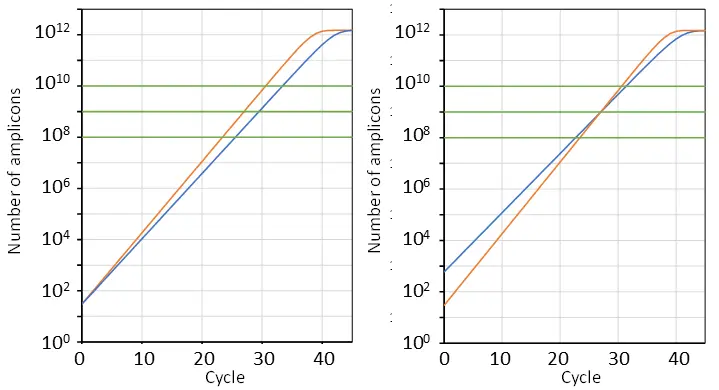
Why Cq alone can mislead in diagnostics
In case of clinical practice, neglecting efficiency and threshold level can have serious consequences. For instance, a reaction with a lower amplification efficiency will take more cycles to reach the quantification threshold, and thus have a higher value, than a reaction with a higher efficiency (Fig. 6, left). In case of diagnostics based on a cut-off value, the reaction with the low efficiency assay may then be erroneously diagnosed as negative. Moreover, when the quantification threshold is set high and the number of cycles in the run is restricted, the reaction with the low efficiency may not even reach the threshold and also be wrongly declared to be negative.
Without standardisation of the setting of the quantification threshold, values cannot be compared, and without including the amplification efficiency in the analysis, values are meaningless. We will discuss this further in a separate blog post.
What the curve can tell you
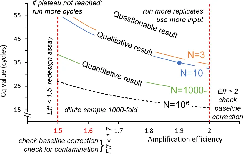
Taken together, the different characteristics of the amplification curves, and the parameters that can be derived from these curves, tell you a great deal about your assay and experiment. Figure 7 summarizes this information for a range of amplification efficiency values (X-axis) and number of targets at the start of the reaction (coloured curves), resulting in a range of values (Y-axis). The text in the graph gives pointers on what to do to optimise the assay or your experimental setup when you find yourself at the extremes of the X-axis and Y-axis of this graph.
Key takeaways
- Inspection of amplification curves gives information on how to optimize the PCR assay and on deviating samples.
- Amplification curves should be inspected on a logarithmic Y-axis to identify the different phases.
- After baseline correction, the cycles in the exponential phase of the PCR should be on a straight line.
- The amplification curves of an assay should show parallel exponential phases; deviating curves indicate inhibitors or stimulators of the PCR.
- All amplification curves should reach the plateau; if not, run more cycles, e.g. 45 cycles.
J.M. Ruijter
Retired Principal Investigator, AMC Amsterdam
Developed methods for 3D analysis and visualization of gene expression patterns during embryogenesis and for the analysis of quantitative PCR data. Creator of LinRegPCR, a widely used method for assumption-free estimation of PCR amplification efficiency.
Maurice van den Hoff
Associate Professor, Amsterdam UMC
Leads a research group focused on the developmental mechanisms of normal and abnormal cardiac development and the molecular response of the diseased heart, in particular after cardiac infarction. With Jan Ruijter, he has worked to improve the reliability of quantitative PCR data analysis.