Every new Clarida workspace comes with this example: a classic two-condition study. Eight subjects were each sampled twice, once untreated and once treated, giving 16 samples in 8 pairs. Four genes of interest were measured against two reference genes, in duplicate, on three plates, together with a dilution series of five standards and a no-template control. Sample and gene names are illustrative.
It is your workspace's copy: colleagues in the workspace see the same one. You can explore every analysis step and change how results are shown; the measured design (samples, targets, plates) is locked so the example stays intact.
How to
1. Open the example and read its goal
Open the paired comparison example: a card on your home page or, once you have an experiment of your own, in the experiment list with the Example badge. The experiment opens on Define: the Background describes the study, and the Goal says what it sets out to answer.
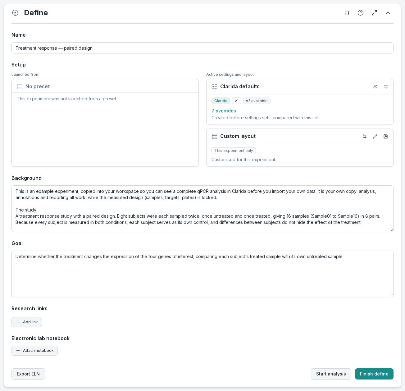
What to notice: scroll down inside the Background box: its last part, Exploring this example, lists the four places this guide visits. Above the experiment, the Demo experiment banner says what you can do: analysis, annotations and reporting all work; structural edits are locked. The Navigator on the side shows where you are, and you can jump to any section from it.
2. See the study design
Go to Design → Sample prep. The list has a column for each sample property: Treatment and Pairing.
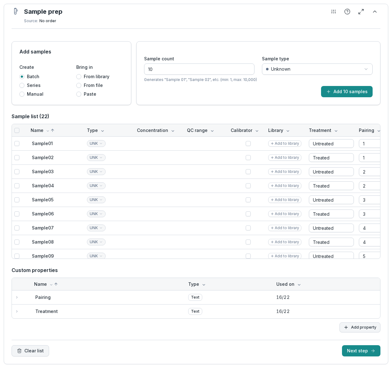
What to notice: each pair number appears twice, once untreated and once treated: Sample01 and Sample02 are subject 1, Sample03 and Sample04 subject 2, and so on. Clarida uses these properties later to group the results, so the design you record here is the design you analyze.
3. Check the amplification efficiency
Go to Analyze → Cq processing → Efficiency. Clarida fits a standard curve through the dilution series of every target and reports its efficiency (E) and the fit (R²). Select a target in the list to see its curve.
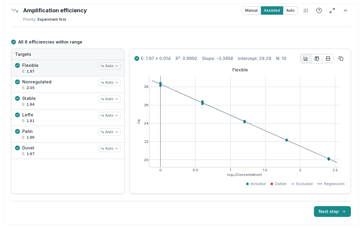
What to notice: each target has its own efficiency, between 1.91 and 2.05 here. Clarida uses each target's own efficiency when it turns Cq values into relative quantities, instead of assuming perfect doubling for every assay. A point that deviates from the curve is marked as an outlier.
4. See what normalization corrects for
Go to Cq processing → Normalization. The table shows the two reference genes with their stability (M and CV); the chart plots the normalization factor of every sample, with a dashed line at 1.
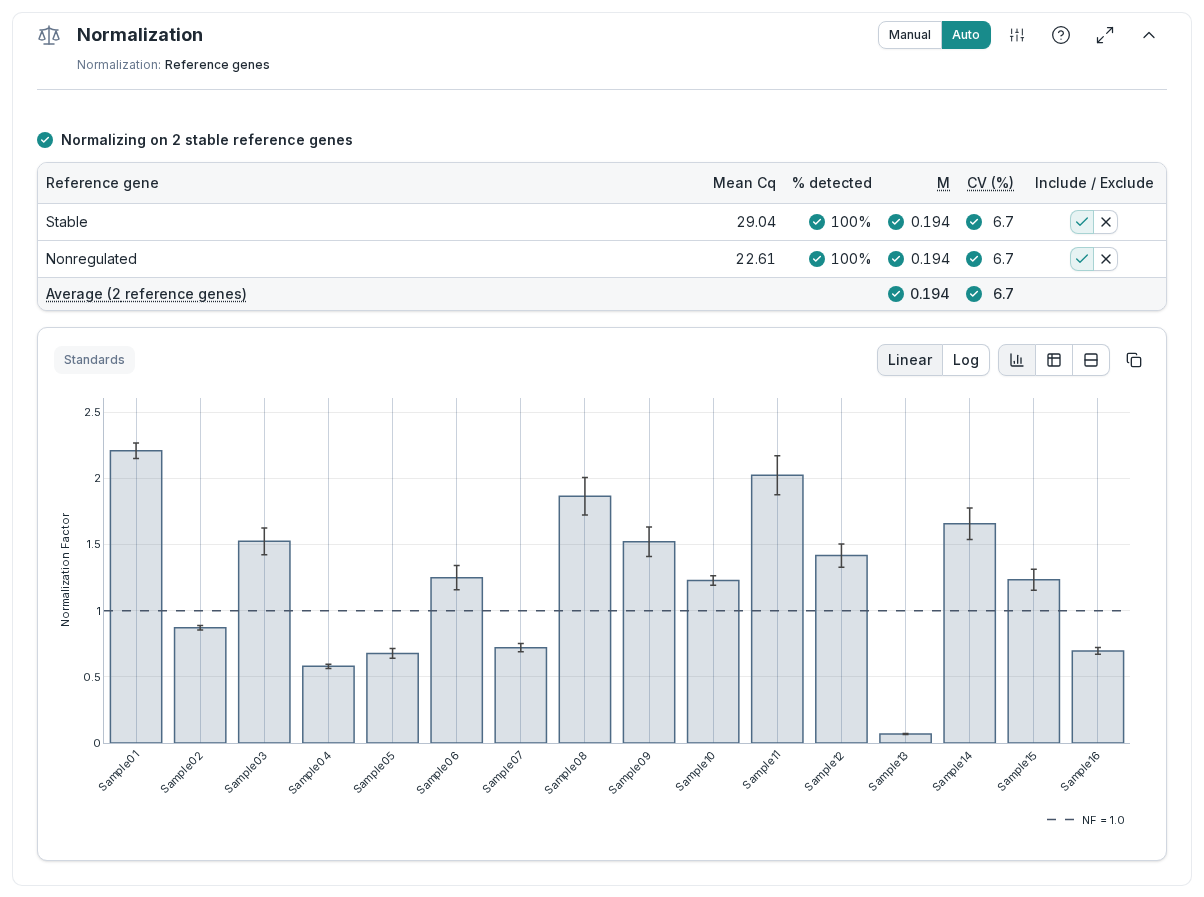
What to notice: the normalization factors range from about 0.07 (Sample13) to about 2.2 (Sample01), so the amount of input differed roughly 30-fold between samples. The two reference genes are stable (green checks on M and CV), so they can be trusted to correct for it.
5. See the result for each pair
Go to Exploration. The Data health summary at the top collects the checks from the previous steps. Below it, the NRQ bar chart shows the first gene. Under Grouping, set Property 1 to Pairing and Property 2 to Treatment.
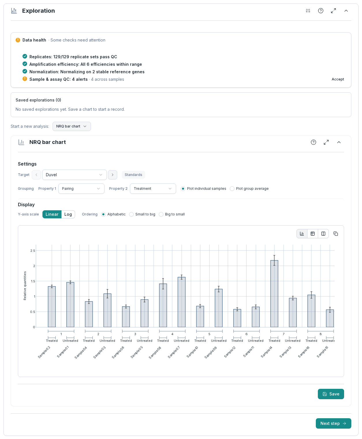
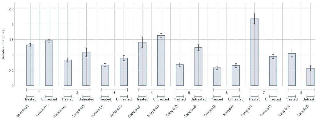
What to notice: each subject now has its own before-and-after comparison. For Duvel, the treated sample is lower than its untreated partner in pairs 1 to 6, and higher in 7 and 8. Seen sample by sample, without the pairing, that pattern is hard to spot: the differences between subjects are larger than the effect of the treatment. That is what a paired design is for: each comparison stays within one subject, so what differs between subjects drops out of it.
The one orange line in Data health, 4 alerts under Sample & assay QC, is the unequal input from step 4. Sample01, Sample11 and Sample13 have normalization factors outside the 0.5 to 2 range, and Sample13, with the least input, also has a high average Cq. Normalization corrects for this. The alerts ask you to take a look at those samples; they don't mean the analysis failed.
6. Test the pairs
Go to Statistics & apps. Next to Start a new analysis, choose Paired t-test. Under Targets, pick Duvel, Flexible, Leffe and Palm. Under Groups, choose Treatment: Treated becomes A and Untreated B. Under Pairing, choose Pairing, and Clarida confirms 8 valid pairs for every gene. Click Analyze, keep the suggested title and click Run: the test is saved, as it ran, in your workspace's copy.
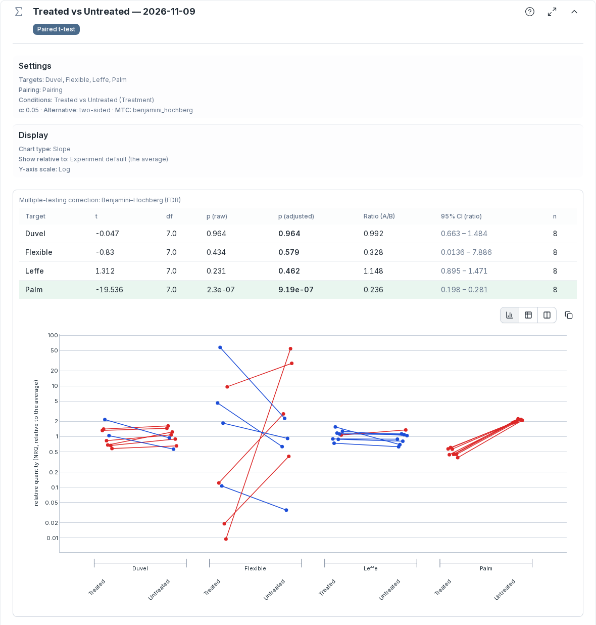
What to notice: only Palm changes with the treatment. Its treated sample is lower in all 8 pairs, a ratio of 0.236 (95% interval 0.198 to 0.281), and its adjusted p-value is far below 0.05, so its row is highlighted. Duvel, lower in 6 of its 8 pairs in step 5, has a ratio of 0.992: the test finds no effect. In the chart, a red line rises to Untreated and a blue line falls.
Try this
With the result in view, change one thing and watch the analysis follow.
- Step through the genes. Use the arrows next to Target to switch to Flexible, Leffe and Palm. Does each gene respond to the treatment the same way in every pair?
- Summarize each group. Switch from Plot individual samples to Plot group average, or set the Y-axis scale to Log. These options change only how the result is shown.
- Test without assuming normality. In the same menu, Wilcoxon signed-rank tests the same pairs on their ranks. It gives a p-value, but no ratio interval.
- Exclude a standard. On Efficiency, click a point on the standard curve and choose Exclude point. E and R² are recalculated, and so is everything downstream. Choose Include point to undo; until you do, the change stays in the workspace's copy, so colleagues see it too.
Exploring qPCR data explains the views of step 5.
What you just did
- Read a study design from its sample properties.
- Checked the amplification efficiency of each assay on its standard curve.
- Saw how reference genes correct for unequal input.
- Viewed the result of a paired experiment pair by pair.
- Tested each gene with a paired t-test.
To do the same on your own run, Importing qPCR run files and Cq (Ct) tables says which exports Clarida reads and how they are matched.