The run file may be on the instrument PC, a network drive or a USB stick. Import it as the instrument saved it: no export, no reformatting.
| From | File | What comes in |
|---|---|---|
| Bio-Rad CFX instruments | .pcrd | Plate layout, amplification and melt curves, instrument Cq |
| Roche LightCycler 480 | .ixo .xml | Plate layout with samples, amplification curves; targets, melt curves and the instrument’s Cq when the file holds them, otherwise Clarida calls Cq |
| Thermo Fisher QuantStudio and ViiA 7 (not the older 7500 and 7900HT files) | .eds | Plate layout, amplification and melt curves, instrument Cq |
| QIAGEN Rotor-Gene | .rex .qrex | Tubes listed by number with their samples, amplification curves, melt curves when run; the file has no Cq, so Clarida calls it |
| RDML The open data standard for qPCR, written by many instruments and tools | .rdml .rdm | Whatever the file holds: annotation, curves, Cq |
| Any instrument A Cq table exported from its software | .xlsx .csv .txt .tsv | Cq values and whatever annotation the table carries; no curves |
Any other instrument: export its Cq table (.xlsx, .csv, .txt or .tsv) with at least a well and a Cq column; sample and target names come along when it has them. Importing qPCR run files and Cq (Ct) tables lists the column names Clarida recognizes.
The screens below show a SYBR Green run from a Bio-Rad CFX96: Actin, IL1Beta and Tubulin, at 0Hr, 1Hr and 2Hr in triplicate, with a dilution series and a no-template control. Follow along with a run of your own.
How to
1. Start an experiment from your file
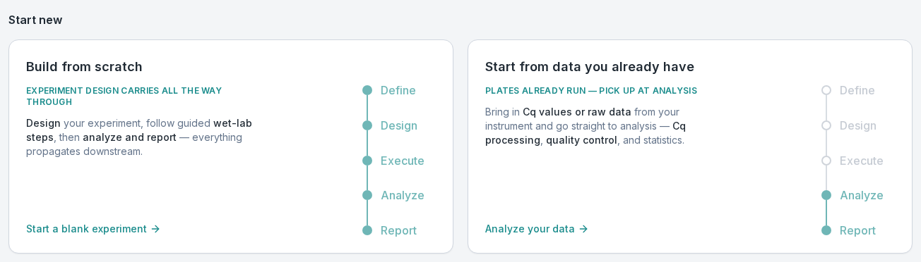
On your home page or the qPCR start page, choose Start from data you already have. The experiment skips Define, Design and Execute, since the file describes the plate, and opens on Analyze → Import & annotate.
2. Drop the run file
Drag the file onto the drop zone, or click it to browse, then choose Parse selected.
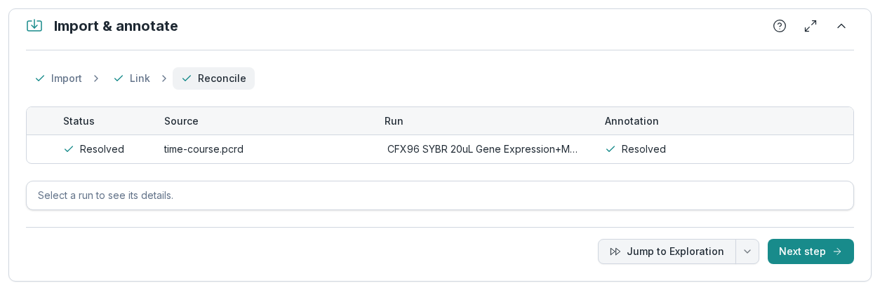
What to notice: Import, Link and Reconcile are all ticked. They check a run against a plate laid out in Clarida; with none, the file's own annotation is used as it is, and the file becomes a run.
3. Check the curves and the imported Cq
Go to Raw data → Amplification, and use the arrows above the chart to step through Actin, IL1Beta and Tubulin. A Cq table has no curves, so this step is for run files.
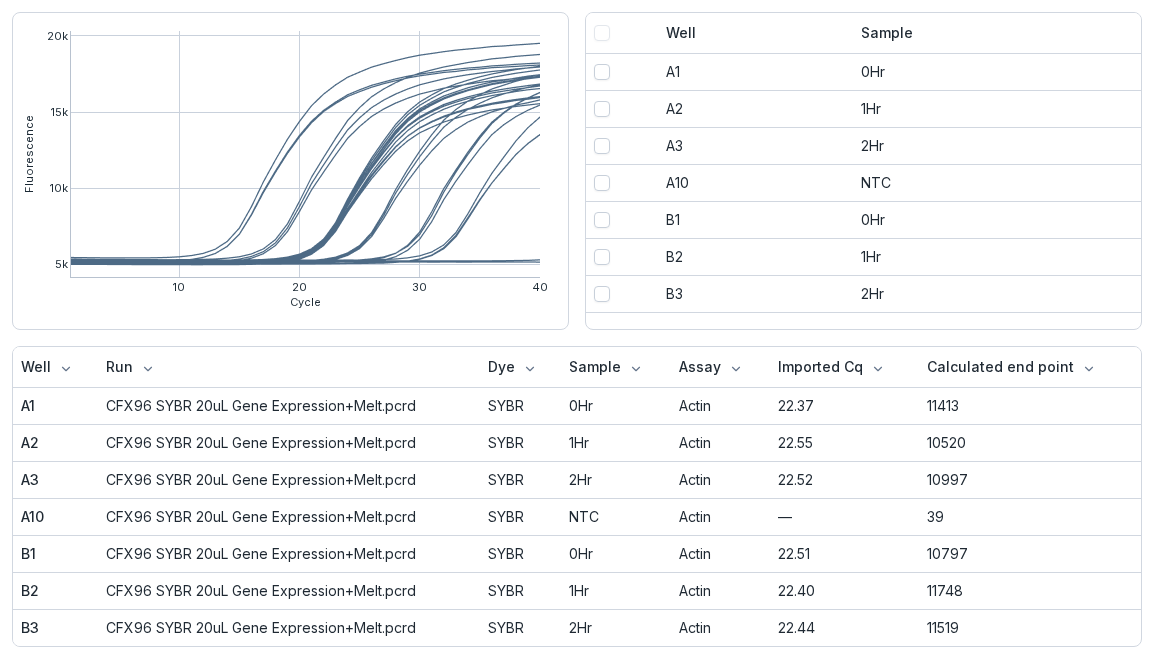
What to notice: the table keeps the Cq your instrument software called, under Imported Cq, and the no-template control (NTC) stays flat. Clarida can call Cq from the curves too, under Cq method; the imported values stay in use until you switch. A Rotor-Gene file holds no Cq, so there Clarida calls it.
4. Check the reference genes
Go to Cq processing → Normalization: the reference genes with their stability, and below them each sample's normalization factor.
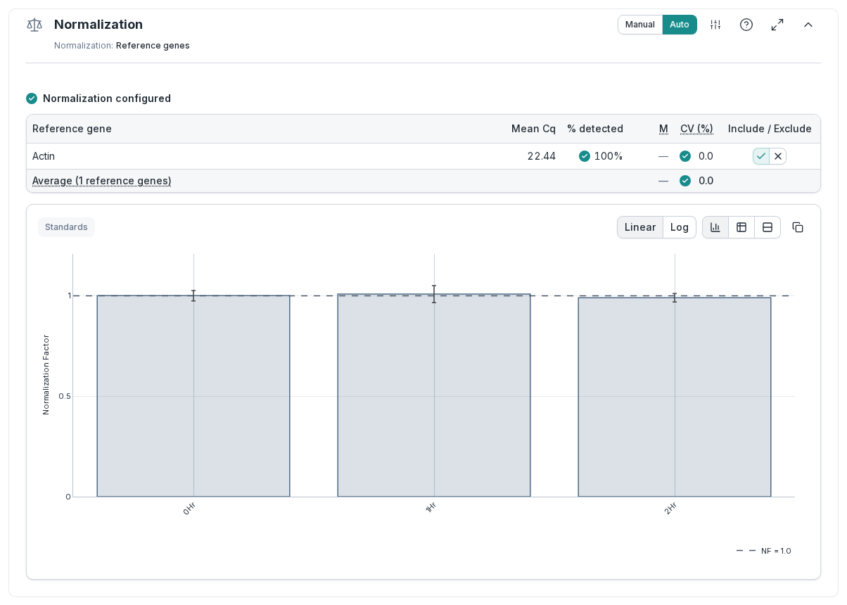
What to notice: the CFX file marked Actin as a reference gene, so the run is normalized on it at once. With one reference gene, M shows a dash, and a CV of 0.0 says nothing about stability: there is no second gene to compare it with.
If the file doesn't name its reference genes (a Cq table and a Rotor-Gene file never do), Normalization lists your targets instead: tick them in the Reference gene column and choose Confirm.
5. Read each target's efficiency
Go to Cq processing → Efficiency and select a target to see its standard curve.
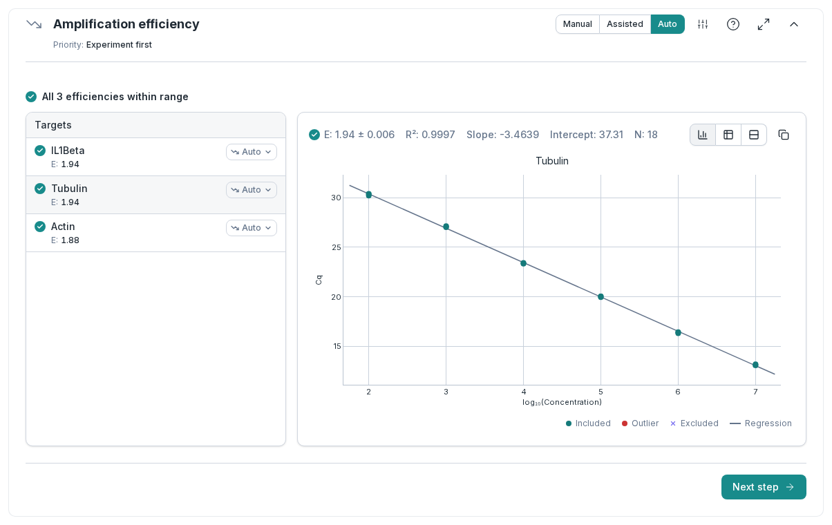
What to notice: each target has its own efficiency, from the run's dilution series: 1.94 for Tubulin and IL1Beta, 1.88 for Actin. Clarida turns Cq into relative quantities with each target's own value, instead of assuming perfect doubling.
6. Read the data health check
Go to Exploration. Data health at the top collects the checks the result rests on; the NRQ bar chart below shows one target at a time.
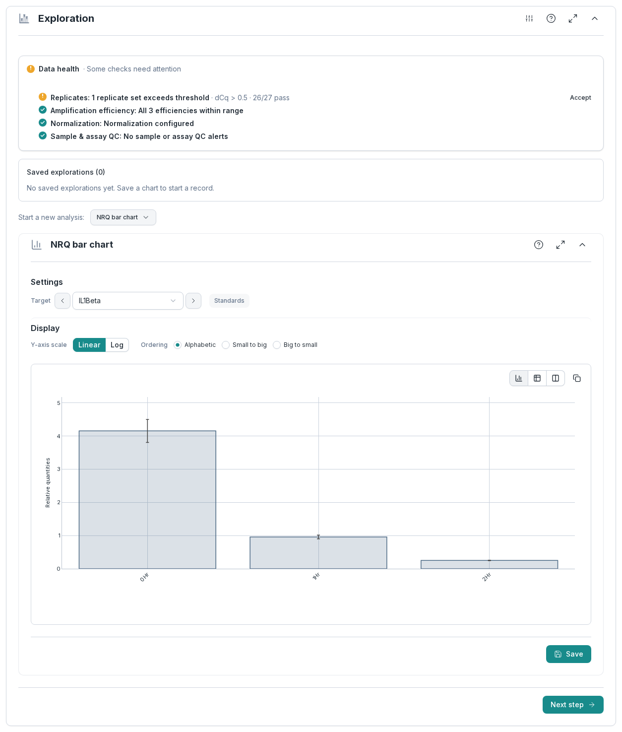
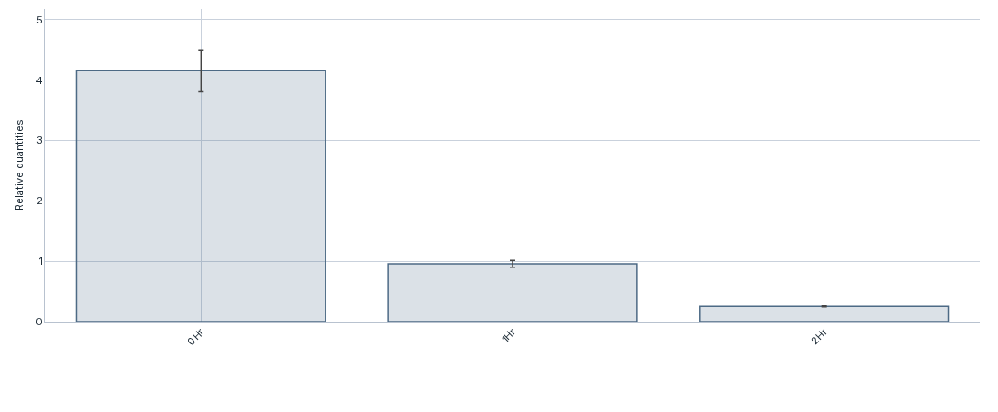
What to notice: one line is orange, 1 replicate set exceeds threshold: an IL1Beta triplicate near Cq 30, its replicates 0.68 cycles apart, above the 0.5 set for this experiment. It asks you to look at that triplicate; it doesn't mean the analysis failed. Use the arrows next to Target to step to IL1Beta, the result in Fig. 1: about four times lower each hour.
Try this
With your own run in view, change one thing and watch the analysis follow.
- Look at the flagged triplicate. Under Cq processing → Replicates, find the IL1Beta set above the threshold, then exclude its deviating well under Cq processing → Exclusion. Data health follows; include the well again to undo it.
- Open the melt curves. When the file holds them, Raw data → Melt shows them.
- Add a second run. Drop another file into Import & annotate, choose Parse selected, then Promote all unlinked (1): the file becomes a second run of the same experiment.
What you just did
- Brought a run into Clarida as your instrument saved it.
- Checked its curves next to the Cq your instrument software called.
- Saw which reference gene it is normalized on, and what one gene can't tell you.
- Read each target's efficiency and the data health of the result.
Which exports Clarida reads, and how a Cq table's columns are matched: Importing qPCR run files and Cq (Ct) tables.